Suppose That an Increase in Income Leads to an Increase in the Demand for Beef. This Means

4.ane Computing Elasticity

Learning Objectives

By the stop of this department, you will be able to:

• Calculate the price elasticity of demand
• Calculate the price elasticity of supply
• Calculate the income elasticity of demand and the cross-price elasticity of need
• Apply concepts of price elasticity to real-globe situations

(Credit: Melo McC/ Flickr/ CC BY-NC-ND 2.0)

That Volition Exist How Much?

Imagine going to your favorite coffee store and having the waiter inform you the pricing has changed. Instead of $3 for a cup of coffee with cream and sweetener, y'all will now exist charged $2 for a black coffee, $ane for creamer, and $one for your choice of sweetener. If you desire to pay your usual $iii for a cup of java, y'all must cull betwixt creamer and sweetener. If you desire both, you now face up an extra charge of $1. Sound cool? Well, that is the state of affairs Netflix customers establish themselves in 2011 – a 60% cost hike to retain the same service.

In early 2011, Netflix consumers paid about $10 a month for a package consisting of streaming video and DVD rentals. In July 2011, the company appear a packaging change. Customers wishing to retain both streaming video and DVD rental would be charged $15.98 per month – a price increase of well-nigh threescore%. In 2014, Netflix also raised its streaming video subscription price from $7.99 to $8.99 per month for new U.S. customers. The company as well changed its policy of 4K streaming content from $nine.00 to $12.00 per month that year.

How did customers of the eighteen-year-old firm react? Did they abandon Netflix? How much volition this price change touch the need for Netflix'south products? The answers to those questions will be explored in this chapter with a concept economists phone call elasticity.

Click to read the residue of the Netflix story

Anyone who has studied economics knows the law of demand: a higher price will atomic number 82 to a lower quantity demanded. What you may not know is how much lower the quantity demanded will be. Similarly, the police force of supply shows that a college price will pb to a college quantity supplied. The question is: How much higher? This topic volition explain how to answer these questions and why they are critically of import in the real world.

To discover answers to these questions, we demand to understand the concept of elasticity.Elasticity is an economics concept that measures the responsiveness of 1 variable to changes in another variable. Suppose yous drib ii items from a second-floor balcony. The starting time detail is a tennis ball, and the second detail is a brick. Which will bounciness higher? Apparently, the tennis ball. We would say that the lawn tennis brawl has greater elasticity.

But how is this degree of responsiveness seen in our models? Both the demand and supply bend show the relationship between cost and quantity, and elasticity can improve our understanding of this human relationship.

Theain cost elasticity of demand is the percent alter in the quantitydemanded of a good or service divided by the percentage alter in the price. This shows the responsiveness of the quantity demanded to a alter in price.

Theain toll elasticity of supply is the percentage change in quantitysupplied divided by the per centum change in price. This shows the responsiveness of quantity supplied to a modify in price.

Our formula for elasticity,[latex]\frac{\%\Delta Quantity}{\%\Delta Price}[/latex], tin can exist used for about elasticity problems, we but utilise dissimilar prices and quantities for different situations.

Why percentages are counter-intuitive

Recall that the simplified formula for percentage change is [latex]\frac{New\;Value-Former\;Value}{Former\;Value}[/latex], also written as [latex]\frac{\Delta Value}{Old\;Value}[/latex].

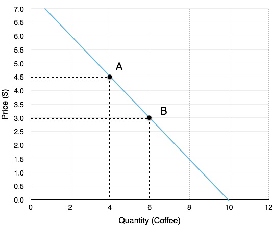
Suppose there is an increase in quantity demanded from 4 coffees to 6 coffees. Calculating percentage change ([latex]\frac{\left(6-four\right)}{4}[/latex]) there has been a 50% increment in quantity demanded. Using the same numbers, consider what happens when quantity demanded decreases from vi coffees to four coffees, ([latex]\frac{\left(four-6\correct)}{6}[/latex]) this modify results in a 33% decrease in quantity demanded.

Right abroad, this should heighten a ruby-red flag about computing the elasticity betwixt at ii points, if pct change is dependant on the direction (A to B or B to A) and then how can we ensure a consistent elasticity value?

Figure 4.1a

Permit'south calculate elasticity from both perspectives:

Moving from A to B:

%ΔPrice: The coffee price falls from $4.l to $3.00, significant the percentage change is [latex]\frac{\left(3.00-iv.50\right)}{4.50}[/latex] = -33%. Price has fallen by 33%.

%ΔQuantity: The quantity of coffee sold increases from 4 to vi, pregnant the percentage alter is [latex]\frac{\left(6-4\right)}{four}[/latex] = 50%. Quantity has risen by fifty%

Elasticity: [latex]\frac{\%\Delta Quantity}{\%\Delta Cost}=-\frac{50\%}{33\%}[/latex] = 1.5*

Moving from B to A:

%ΔPrice: The java toll rises from $iii.00 to $4.fifty, meaning the percentage change is [latex]\frac{\left(4.50-3.00\correct)}{3.00}[/latex] = 50%. Cost has risen by l%.

%ΔQuantity:
The quantity of coffee sold falls from 6 to 4, meaning the pct change is [latex]\frac{\left(4-6\right)}{6}[/latex] = -33%. Quantity has fallen by 33%

Elasticity:  [latex]\frac{\%\Delta Quantity}{\%\Delta Price}=\frac{33\%}{50\%}[/latex] = 0.67

These two calculations requite usa different numbers. This type of analysis would make elasticity subject area to direction which adds unnecessary complication. To avoid this, we will instead rely on averages.

*Note that elasticity is an absolute value, meaning it is non affected by positive of negative values.

Mid-point Method

To summate elasticity, instead of using simple percentage changes in quantity and price, economists utilise the boilerplate percent change. This is called the mid-point method for elasticity, and is represented in the following equations:

[latex]\begin{array}{r @{{}={}} l}\%\;change\;in\;quantity & \frac { { Q }_{ 2 }-{ Q }_{ one } }{ ({ Q }_{ ii }+{ Q }_{ 1 })/2 } \times 100 \\[1em] \%\;change\;in\;toll & \frac { { P }_{ 2 }-{ P }_{ 1 } }{ ({ P }_{ 2 }+{ P }_{ 1 })/2 } \times 100 \end{array}[/latex]

The advantage of the chiliad id-point method is that 1 obtains the same elasticity between two cost points whether at that place is a price increase or decrease. This is because the denominator is an average rather than the sometime value.

Using the mid-point method to calculate the elasticity between Bespeak A and Point B:

[latex]\begin{array}{r @{{}={}} fifty}\%\;alter\;in\;quantity & \frac { { 6 }-{ 4 } }{ ({ vi }+{ 4 })/2 } \times 100 \\[1em] & \frac { 2 }{ v } \times 100 \\[1em] & 40\% \\[1em] \%\;change\;in\;price & \frac { { 3.00 }-{ 4.50 } }{ ({ 3.00 }+{ 4.50 })/ii } \times 100 \\[1em] & \frac { -1.50 }{ 3.75 } \times 100 \\[1em] & -xl\% \\[1em] Price\;Elasticity\;of\;Demand & \frac { twoscore\% }{ 40\% } \\[1em] & 1 \end{array}[/latex]

This method gives us a sort of average elasticity of demand over 2 points on our curve. Notice that our elasticity of 1 falls in-between the elasticities of 0.67 and 1.52 that nosotros calculated in the previous example.

Betoken-Gradient Formula

In Figure 4.1a we were given two points and looked at elasticity every bit movements along a bend. As we will meet in Topic four.three, it is often useful to view elasticity at a single point. To calculate this, we accept to derive a new equation.

[latex]\frac{\%\Delta Quantity}{\%\Delta Toll}=Elasticity[/latex]

Since nosotros know that a pct modify in price can be rewritten equally

[latex]\frac{\Delta Price}{Price}[/latex]

and a percentage change in quantity to

[latex]\frac{\Delta Quantity}{Quantity}[/latex]

we can rearrange the original equation as

[latex]\frac{\frac{\Delta Quantity}{Quantity}}{\frac{\Delta Cost}{Price}}[/latex]

which is the same every bit saying

[latex]\frac{\Delta Quantity\cdot Price}{\Delta Price\cdot Quantity}=\frac{\Delta Q}{\Delta P}\cdot \frac{P}{Q}[/latex]

This gives us our betoken-gradient formula. How do we use it to calculate the elasticity at Point A? The P/Q portion of our equation corresponds to the values at the point, which are $4.5 and 4. The ΔQ/ ΔP corresponds to thechanged slope of the curve.Recollect slope is calculated as rise/run.

In Effigy four.ane, the slope is [latex]\frac{3-4.five}{6-4}[/latex] = 0.75, which means the inverse is 1/0.75 = 1.33. Plugging this information into our equation, we become:

[latex]\frac{\Delta Q}{\Delta P}\cdot \frac{P}{Q}[/latex]

[latex]one.33\cdot \frac{4.5}{four}[/latex] = 1.5

This analysis gives usa elasticity as a single signal. Discover that this gives us the aforementioned number as calculating elasticity from Indicate A to B. This is non a coincidence. When we are calculating from Indicate A to Indicate B, we are actually just calculating the elasticity at Point A, since we are using the values on Point A as the denominator for our percent change. Likewise from Signal B to Indicate A, we are calculating the elasticity at Betoken B. When nosotros use the mid-indicate method, nosotros are just taking an average of the ii points. This solidifies the fact that at that place is a unlike elasticity at every point on our line, a concept that will be important when we discuss acquirement.

Non Actually So Different

Even though mid-point and Point-Slope appear to exist adequately different formulas, mid-indicate tin can be rewritten to testify how like the 2 really are.

[latex]\frac{\frac{\Delta Q}{(Q1+Q2)/2}}{\frac{\Delta P}{(P1+P2)/ii}}[/latex] = [latex]\frac{\frac{\Delta Q}{Q1+Q2}}{\frac{\Delta P}{P1+P2}}[/latex]

Retrieve that when a fraction is divided by a fraction, you can rearrange information technology to a fraction multiplied past the inverse of the denominator fraction.

= [latex]\frac{\Delta Q}{\Delta P}\cdot \frac{\left(P1+P2\right)}{\left(Q1+Q2\correct)}[/latex]

Notice that compared to bespeak-slope: [latex]\frac{\Delta Q}{\Delta P}\cdot \frac{P}{Q}[/latex], the simply difference is that bespeak-gradient is the inverse of the slope multiplied by a single signal, whereas mid-point is the inverse of the gradient multiplied by multiple points. This reinforces the conclusion that mid-point represents an average.

Other Elasticities

Call up, elasticity is the responsiveness of one variable to changes in another variable. This means it can be applied to more than that simply the price-quantity relationship of our market model. In Topic 3 we discussed how goods can be inferior/normal or substitutes/complements. We volition examine this fifty-fifty further when nosotros innovate consumer theory, but for now we tin develop our understanding by applying what we know about elasticities.

Own-toll elasticity of supply (due east_P ^South)

Our assay of elasticity has been centred effectually demand, just the same principles apply to the supply bend. Whereas elasticity of demand measures responsiveness of quantity demanded to a price alter, own-price elasticity of supplymeasures the responsiveness of quantity supplied. The more rubberband a firm, the more information technology tin can increase production when prices are rising, and subtract its production when prices are falling. Our equation is equally follows:

[latex]\frac{\%\Delta Q\;Supplied}{\%\Delta P}[/latex]

Own-toll elasticity of supply can be calculated using mid-point and point-gradient formula in the same way every bit for e_P ^D.

Cross-price elasticity of demand (due east_XP ^D)

Whereas the own-price elasticity of need measures the responsiveness of quantity to a goods own price, cantankerous-price elasticity of demand shows u.s.a. how quantity demand responds to changes in the price ofrelatedgoods. Whereas before we could ignore positives and negatives with elasticities, with cross-toll, this matters. Our equation is equally follows:

[latex]\frac{\%\Delta Q\;Practiced A}{\%\Delta P\;Good B}[/latex]

Consider our discussion of complements and substitutes in Topic 3.3. We defined complements as goods that individuals prefer to consume with another good, and substitutes as appurtenances individuals adopt to consume instead of another practiced. If the price of a complement rises our demand will autumn, if the toll of a substitute rises our need will rise. For cross-toll elasticity this means:

A complement will have a negative cross-price elasticity, since if the % change in cost is positive, the % change in quantity volition exist negative and vice-versa.

A substitute will have a positive cross-price elasticity, since if the % alter in price is positive, the % change in quantity will be positive and vice-versa.

This adds another dimension to our give-and-take of complements/substitutes. At present we tin comment on the strength of the human relationship between two appurtenances. For example, a cross-price elasticity of -4 suggests an individual strongly prefers to consume two appurtenances together, compared to a cross-cost elasticity of -0.v. This could represent the cross-price elasticity of a consumer for a hot dog, with respect to ketchup and relish. The consumer might strongly prefer to consume hot dogs with ketchup, and loosely prefers relish.

Income elasticity of demand (e_N ^D)

In Topic 3 we also explained how goods can be normal or inferior depending on how a consumer responds to a change in income. This responsiveness tin can as well be measured with elasticity by the income elasticity of demand.Our equation is as follows:

[latex]\frac{\%\Delta Q}{\%\Delta Income}[/latex]

As with cross-price elasticity, whether our elasticity is positive or negative provides valuable information well-nigh how the consumer views the good:

A normal skillful will have a positive income elasticity, since if the % change in income is positive, the % modify in quantity will be positive and vice-versa.

A junior good volition accept a negative income elasticity, since if the % change in income is positive, the % change in quantity will be negative and vice-versa.

The value of our elasticity will bespeak how responsive a good is to a change in income. A adept with an income elasticity of 0.05, while technically a normal good (since demand increases after an increment in income) is not near every bit responsive every bit one with an income elasticity of need of 5.

Summary

Elasticity is a measure out of responsiveness, calculated by the percentage change in ane variable divided by the per centum change in some other.

Both mid-betoken and point-slope formulas are of import for calculating elasticity in dissimilar situations. Mid-point gives an average of elasticities between two points, whereas signal-slope gives the elasticity at a certain point. These can be calculated with the post-obit formulas:

Base of operations Formula	Mid-Point Formula	Betoken-Slope Formula
[latex]\frac{\%\Delta Quantity}{\%\Delta Toll}[/latex]	[latex]\frac{\Delta Q}{\Delta P}\cdot \frac{\left(P1+P2\right)}{\left(Q1+Q2\right)}[/latex]	[latex]\frac{\Delta Q}{\Delta P}\cdot \frac{P}{Q}[/latex]

Since elasticity measures responsiveness, information technology tin also exist used to mensurate the own-price elasticity of supply, the cantankerous-toll elasticity of demand, and the income elasticity of need. These can be calculated with the following formulas:

Own-Price Elasticity of Supply	Cantankerous-Toll Elasticity of Demand	Income Elasticity of Demand
[latex]\frac{\%\Delta Q\;Supplied}{\%\Delta P}[/latex]	[latex]\frac{\%\Delta Q\;Skilful A}{\%\Delta P\;Good B}[/latex]	[latex]\frac{\%\Delta Q}{\%\Delta Income}[/latex]

Glossary

Cross-price elasticity of demand

the pct modify in the quantity demanded of skilful A as a result of a pct change in price of adept B

Elasticity

an economics concept that measures responsiveness of ane variable to changes in another variable

Income elasticity of need

the per centum modify in quantity demanded of a good or service equally a result of a percentage alter in income

Own-price elasticity of need

percentage change in the quantity demanded of a good or service divided the percentage change in price

Mid-point Method

Involves multiplying the inverse of the slope by the values of a single bespeak.

Own-price elasticity of supply

percentage modify in the quantity supplied divided past the percentage change in toll

Point Gradient Method

A method of computing elasticity betwixt two points. Involves calculating the percentage modify of price and quantity with respect to an average of the two points.

Exercises 4.1

1. Use the demand curve diagram below to reply the post-obit question.

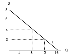
What is the ain-cost elasticity of need as toll increases from $ii per unit to $four per unit of measurement? Use the mid-indicate formula in your calculation.

a) 1/3.
b) 6/10.
c) 2/iii.
d) None of the above.

2. Suppose that a 2% increment in cost results in a 6% decrease in quantity demanded. Ain-price elasticity of demand is equal to:

a) 1/3.
b) 6.
c) two
d) iii.

3. If own-cost elasticity of demand equals 0.3 in absolute value, and then what percentage modify in cost will result in a vi% decrease in quantity demanded?

a) three%
b) 6%
c) 20%.
d) 50%.

four. Suppose y'all are told that the own-cost elasticity of supply equal 0.5. Which of the post-obit is the right interpretation of this number?

a) A ane% increase in price volition result in a l% increase in quantity supplied.
b) A 1% increase in price will issue in a 5% increase in quantity supplied.
c) A ane% increase in price volition result in a 2% increase in quantity supplied.
d) A ane% increment in toll will result in a 0.5% increase in quantity supplied.

5. Suppose that a x increase in price results in a 50 percent decrease in quantity demanded. What does (the absolute value of) own price elasticity of need equal?

a) 0.5.
b) 0.two.
c) v.
d) 10.

vi. If appurtenances 10 and Y are SUBSTITUTES, then which of the post-obit could be the value of the cantankerous cost elasticity of demand for good Y?

a) -1.
b) -2.
c) Neither a) nor b).
d) Both a) and b).

seven. If pizza is a normal good, so which of the following could be the value of income elasticity of demand?

a) 0.2.
b) 0.8.
c) 1.4
d) All of the above.

8. If goods X and Y are COMPLEMENTS, the which of the following could exist the value of cantankerous cost elasticity of demand?

a) 0.
b) 1.
c) -1.
d) All of the above could exist the value of cross price elasticity of need.

valentinasaing74.blogspot.com

Source: https://pressbooks.bccampus.ca/uvicecon103/chapter/4-2-elasticity/